15 October 2026
A common structure in specialty finance buys a pool of consumer loans at a price near par and finances most of it by issuing senior and mezzanine notes, keeping the residual as equity. We study a stylised, fully synthetic version of this structure as an applied-mathematics problem. We build a loan-level cash-flow engine with correlated defaults (a one-factor Vasicek model) and a sequential-pay waterfall with an overcollateralisation test and cash trap. We then prove and numerically verify three exact results. (i) A pool of identical loans bought at par has an internal rate of return that satisfies a closed-form fixed-point equation and is independent of the prepayment rate; the same identity extends loan by loan to heterogeneous pools and gives closed-form sensitivities and a pull-to-par price sensitivity. (ii) The equity IRR of a levered pool is exact under a single note and, with the right bookkeeping, under two sequential-pay notes; leverage amplifies price sensitivity by a factor we compute exactly (\(5.8\times\) at an 80% advance rate, against the naive \(5\times\)). (iii) The one-year loss law of a large pool is Vasicek’s, and for lifetime losses a one-parameter saturating form \(C=p/(\theta+p)\) reproduces the engine’s loss quantiles to within 1–5% where the linear form errs by up to 36%. We quantify how much the closed-form senior advance rate understates the engine’s by ignoring excess spread (7 to 13 percentage points in our grid), and how a pool of 25 loans has a 99th-percentile default fraction 49% above its large-pool limit. Finally we map the equity value against purchase price and leverage, locate the break-even price (it rises about 0.11 points per point of advance rate), and use one-at-a-time elasticities and a 240-point Latin-hypercube study to rank the drivers of the arbitrage. All results are model-based and use no real loan data.
Consider an investor who buys a pool of fixed-rate consumer loans at a price \(P\) close to par and finances it by issuing two classes of notes against the pool: a senior note \(A\) with a low coupon and a mezzanine note \(B\) with a higher one. The investor keeps the residual interest (the equity). If the pool yields more than the blended cost of the notes, the equity earns a levered return, and the question of how much the buyer can afford to pay for the loans becomes a question about the securitization. This is sometimes called a securitization arbitrage: the loans are worth more as a financed pool than as whole loans bought with the investor’s own cash.
This paper takes that structure seriously as a mathematical object. Our aims are:
to separate what can be said exactly from what must be simulated;
to give simple closed forms, with their accuracy measured, for the quantities a structurer needs, such as the pool’s loss distribution and the largest senior advance rate;
to say, with measured uncertainty, which assumptions drive the value of the equity.
Data. Everything here is synthetic. The loan tape is generated by a random-number routine (Section 2), the assumptions are generic, and no third-party or confidential data are used. The quantitative statements are therefore statements about a model, and we make no claim about any real transaction, market or institution.
Exact pool yield (Section 3). For identical loans the pool IRR solves \(y=y_0(y)\) with \(y_0\) explicit; at par the prepayment rate drops out entirely. We verify it against the engine to \(8\times10^{-12}\) across 300 random parameter sets and extend it exactly to heterogeneous pools.
Exact levered equity (Section 3). Equity IRR under one note and under two sequential-pay notes is given by an explicit equation, verified to \(10^{-11}\). Leverage amplifies the price sensitivity of the equity IRR to \(5.83\times\) that of the pool at an 80% advance rate.
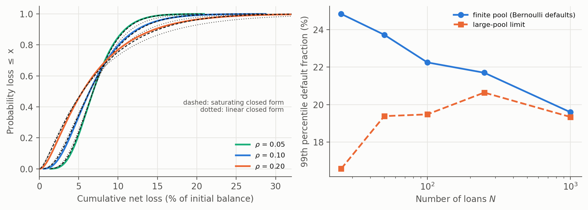
Credit risk (Section 4). A finite pool has fatter tails than the large-pool limit: 49% higher 99th-percentile default fraction at 25 loans, 14% at 100, 1.6% at 1 000. A saturating closed-form loss law fits the engine’s loss quantiles to within 1–5%.
The arbitrage (Sections 5 and 6). The base case has median equity IRR 26% and a 12% chance that equity loses money, and neither note loses principal. The break-even price rises about 0.11 points per point of advance rate. The dominant drivers of equity value are default rate, coupons and the hurdle rate; prepayment speed is nearly irrelevant near par, as the exact identity predicts.
A pool has \(N\) fixed-rate level-pay loans \(k=1,\dots,N\) with current balance \(B_k\), monthly rate \(i_k\) (APR\(/12\)) and remaining term \(n_k\) months. The synthetic tape draws a credit score from a normal law, makes the APR a decreasing function of score plus noise, and makes the annual default probability \(p_k\) a decreasing function of score, scaled so the balance-weighted mean is \(\bar p\). The tape used throughout has \(N=1000\) loans, $10.8 million of balance, a weighted-average APR of \(18.6\%\) and weighted-average remaining term \(34.9\) months.
Loan \(k\) defaults at a constant monthly rate \(m_k\), prepays at a constant monthly rate \(s\) (the single monthly mortality, \(s=1-(1-\mathrm{CPR})^{1/12}\)), and the pool pays a servicing fee of \(\sigma\) per year on the beginning balance. In month \(t\) let \(B_{k,t-1}\) be the beginning balance. Then \[\begin{align*} \text{defaults } d_{k,t} &= m_k B_{k,t-1}, & \text{performing balance } &= (1-m_k)B_{k,t-1},\\ \text{interest } &= i_k(1-m_k)B_{k,t-1}, & \text{scheduled principal } &= (1-m_k)B_{k,t-1}\,\frac{i_k}{(1+i_k)^{n_k-t+1}-1},\\ \text{prepayment } &= s\,(\text{performing}-\text{scheduled}), & \text{servicing } &= \tfrac{\sigma}{12}B_{k,t-1}, \end{align*}\] and a fraction \(R\) of each default is recovered \(\ell\) months later. The pool’s cash flow in month \(t\) is interest plus principal plus recoveries minus servicing.
Defaults share a single systematic factor \(z\sim\mathcal N(0,1)\), held fixed over the pool’s life (a static scenario). Conditional on \(z\), loan \(k\) has annual default probability \[p_k(z)=\Phi\!\left(\frac{\Phi^{-1}(p_k)-\sqrt{\rho}\,z}{\sqrt{1-\rho}}\right),\qquad m_k(z)=1-\bigl(1-p_k(z)\bigr)^{1/12},\] where \(\rho\) is the asset correlation (Vasicek’s one-factor model [1]). Low \(z\) means a bad economy. Averaging over \(z\) is done with an equal-probability quantile grid \(z_j=\Phi^{-1}\bigl((j-\tfrac12)/S\bigr)\), which makes every number below deterministic and reproducible; the engine is vectorised over scenarios and runs 400 scenarios on 1 000 loans in about a second. Conditional on \(z\) the pool is deterministic (the large-pool limit); idiosyncratic randomness is studied separately in Section 4.
Notes \(A\) and \(B\) are issued at par with initial balances \(\alpha_A U\) and \((\alpha_B-\alpha_A)U\), where \(U\) is the initial pool balance and \(\alpha_A<\alpha_B\) are advance rates, at coupons \(c_A<c_B\). The equity cheque is \[E=(P+\kappa-\alpha_B)\,U,\] where \(\kappa\) is an acquisition and structuring cost. Each month the waterfall (i) pays interest on \(A\), then on \(B\), capitalising any shortfall; (ii) pays principal, first to \(A\) and then to \(B\), to restore the debt to the target \(D_t\le\alpha_B\,\mathrm{Bal}_t\) against the current collateral balance; (iii) releases the remaining cash to equity unless the target was missed in the previous month, in which case all cash is trapped and sweeps to the notes; and (iv) at the final month sweeps everything to the notes. Principal still owed after the last month is a loss to the note. The model has no interest-rate or basis risk and no triggers other than this overcollateralisation test.
For each scenario we compute the equity IRR, the pool’s unlevered IRR at price \(P\), and each note’s terminal shortfall as a fraction of its initial balance. Equity value is measured by the NPV of its cash flows at an annual hurdle \(h\), minus the cheque \(E\), per unit of \(U\). The break-even price \(P^*(\alpha_B)\) is the price at which the mean equity NPV is zero.
| Quantity | Symbol | Base value |
|---|---|---|
| Purchase price (fraction of balance) | \(P\) | 1.00 |
| Annual prepayment rate | CPR | 0.15 |
| Mean annual default probability | \(\bar p\) | 0.07 |
| Asset correlation | \(\rho\) | 0.10 |
| Recovery rate; lag | \(R\); \(\ell\) | 0.20; 3 months |
| Servicing fee (annual) | \(\sigma\) | 0.01 |
| Advance rates: senior; total | \(\alpha_A\); \(\alpha_B\) | 0.60; 0.80 |
| Coupons: senior; mezzanine | \(c_A\); \(c_B\) | 0.065; 0.105 |
| Acquisition cost | \(\kappa\) | 0.01 |
| Equity hurdle (annual) | \(h\) | 0.20 |
Consider first a pool of identical loans (monthly rate \(i\), same remaining term, default rate \(m\), prepayment rate \(s\), servicing \(\sigma_m=\sigma/12\)). Let \(B_t\) be the pool balance after month \(t\) and \(G(v)=\sum_{t\ge0}B_tv^t\).
For discount factor \(v=1/(1+y)\) the present value of the pool’s cash flows is \[\mathrm{PV}(v)=B_0+\bigl[(1+y_0(v))\,v-1\bigr]G(v),\qquad y_0(v)=i(1-m)-m\bigl(1-Rv^{\ell}\bigr)-\sigma_m .\] The IRR \(y\) at price \(P\) is the root of \(\mathrm{PV}(v)=PB_0\). At par it solves the fixed-point equation \(y=y_0\bigl(\tfrac{1}{1+y}\bigr)\).
Proof. In month \(t\) the pool pays interest \(i(1-m)B_{t-1}\), collected principal \(B_{t-1}-B_t-mB_{t-1}\), recoveries \(RmB_{t-1-\ell}\), and servicing \(\sigma_mB_{t-1}\), so its cash flow is \(c_t=\bigl[i(1-m)-m-\sigma_m\bigr]B_{t-1}+(B_{t-1}-B_t)+RmB_{t-1-\ell}\). Multiply by \(v^t\) and sum. The balance-change terms telescope: \(\sum_{t\ge1}(B_{t-1}-B_t)v^t=B_0+(v-1)G(v)\). The terms in \(B_{t-1}\) sum to \(v\,G(v)\), and the recovery terms to \(v^{\ell+1}G(v)\). Collecting gives the formula. At \(P=1\) the condition \(\mathrm{PV}=B_0\) holds for \(G>0\) exactly when \((1+y_0)v=1\). \(\square\)
The prepayment rate enters \(\mathrm{PV}\) only through \(B_t\), hence only through \(G(v)\), and \(G\) multiplies a bracket that vanishes at par. So the IRR of a pool bought at par does not depend on the prepayment speed. Numerically, the engine’s pool IRR is identical to 17 digits for CPR from 0% to 45% (\(12.74\%\) in each case at an APR of 19% and a default probability of 7%).
Differentiating \(y=y_0(y)\) implicitly at par gives \[\frac{\partial y}{\partial\theta}=\frac{\partial y_0/\partial\theta}{1+mR\ell\,v^{\ell+1}},\qquad \frac{\partial y_0}{\partial m}=-(1+i-Rv^\ell),\quad \frac{\partial y_0}{\partial R}=mv^\ell,\quad \frac{\partial y_0}{\partial\sigma_m}=-1,\quad \frac{\partial y_0}{\partial i}=1-m .\] With no recovery lag the denominator is \(1\) and the sensitivities are those of a simple coupon-minus-loss yield. These match finite differences of the exact solution with relative error below \(10^{-7}\) in every case tested.
Away from par, \(\mathrm{PV}(v)=PB_0\) gives \(y=y_0+(1-P)(1+y)/g(v)\) with \(g=G/B_0\). The price sensitivity is therefore, to leading order, \(\partial y/\partial P\approx-(1+y)/g\): the reciprocal of a duration measured in months. In the base pool \(g/(1+y)=15.5\) months, giving \(\partial y/\partial P\approx-0.0645\) per unit of price against \(-0.0643\) from the exact solution (a \(0.3\%\) difference). Equivalently, a one-point change in price moves the pool’s monthly yield by about \(0.00064\).
The identity holds loan by loan, so \(\mathrm{PV}_{\text{pool}}(v)=\sum_k\mathrm{PV}_k(v)\) with each loan’s own \((i_k,m_k,B_{k,t})\). The pool IRR is the root of this sum. We re-implemented the balance recursion independently and compared with the engine on 21 combinations of scenario and price: the largest IRR difference is \(3\times10^{-14}\).
Suppose the notes are held at \(D_t=\alpha_BB_t\) with no shortfall and no cash trap, and that the notes \(A\) (coupon \(c_A\)) and \(B\) (coupon \(c_B\)) are paid sequentially, so that \(B\) is untouched until \(A\) is retired: \(A_t=\max(D_t-b,0)\) with \(b=(\alpha_B-\alpha_A)B_0\) and \(B_t=D_t-A_t\). Then the equity IRR is the root of \[\mathrm{PV}_{\text{pool}}(v)-\sum_{t\ge1}v^t\Bigl[\tfrac{c_A}{12}A_{t-1}+\tfrac{c_B}{12}B_{t-1}+(D_{t-1}-D_t)\Bigr]=(P+\kappa-\alpha_B)B_0 .\] Proof. Equity cash flow equals pool cash flow minus debt service, and both present values are explicit. \(\square\)
With a single note of coupon \(c\), no lag, and \(P+\kappa=1\), equity cash flow becomes \(\frac{y_0-c\alpha}{1-\alpha}E'_{t-1}+(E'_{t-1}-E'_t)\) with \(E'_t=(1-\alpha)B_t\), a par bond with coupon equal to its IRR, which gives the leverage identity (all rates monthly) \[y_E=\frac{y_0-c\,\alpha}{1-\alpha}=y_0+\frac{\alpha}{1-\alpha}\,(y_0-c).\] Proposition 3 shows what the identity hides when there are two notes: since \(A\) amortises first, the blended cost of funds drifts up over the pool’s life as the pricier \(B\) becomes a larger share of the debt. Using a constant blended coupon instead of the exact path gives a median IRR error of 1.1 percentage points (95th percentile 6.5) in our tests.
To first order a price change is spread over an equity cheque that is only a fraction \(1-\alpha_B\) of the pool, so the equity IRR should move about \(1/(1-\alpha_B)\) times as much as the pool’s. For \(\alpha_B=0.8\) this naive factor is \(5\). The exact figure from Proposition 3, computed in the no-loss path with \(\alpha_A=0.6\), is \(5.83\): the equity’s yield is a bit more price-sensitive than the first-order argument suggests.
| Identity (random parameter sets) | Cases | Max. IRR error |
|---|---|---|
| Pool yield, any price, lag and CPR (Prop. 1) | 300 | \(7.5\times10^{-12}\) |
| Pool yield, heterogeneous pool (Prop. 2) | 21 | \(3.0\times10^{-14}\) |
| Equity, single note (Prop. 3, special case) | 300 | \(9.8\times10^{-12}\) |
| Equity, two sequential notes (Prop. 3) | 300 | \(1.0\times10^{-11}\) |
| Implicit derivatives (Cor. 2), max. relative error | 120 | \(8.8\times10^{-8}\) |
The engine conditions on \(z\) and ignores idiosyncratic default randomness. For a pool of \(N\) loans the one-year default fraction is \(X_N=\sum_kw_k\mathbf 1\{\text{loan }k\text{ defaults}\}\) with weights \(w_k=B_k/\sum B\), and the large-pool limit \(\sum_kw_kp_k(z)\) drops the Bernoulli noise. Gordy [2] studied this gap as the granularity adjustment. We measure it on random sub-pools drawn from the tape, comparing each with its own large-pool limit.
| Loans \(N\) | Effective \(N\) | 99th pct, finite | 99th pct, limit | Excess |
|---|---|---|---|---|
| 25 | 19 | 24.8% | 16.6% | +49% |
| 50 | 39 | 23.7% | 19.4% | +22% |
| 100 | 66 | 22.3% | 19.5% | +14% |
| 250 | 175 | 21.7% | 20.6% | +5% |
| 1000 | 706 | 19.6% | 19.3% | +1.6% |
The excess comes from idiosyncratic randomness and shrinks roughly in proportion to \(1/N_{\text{eff}}\): the variance of the default fraction exceeds its large-pool value by \(0.0023\) at \(N=25\) (standard deviations \(0.059\) against \(0.034\)) and by \(0.0003\) at \(N=250\) (\(0.045\) against \(0.041\)). The loan-level engine in Sections 5–6 uses 1 000 loans, where the limit is accurate to about 2%.
Given \(z\), the pool’s annual default rate is \(p(z)\). The cumulative default fraction over the pool’s life depends on how long the balance survives. If the balance runs off at an effective annual rate \(\theta\) (amortisation and prepayment), and defaults draw it down at rate \(p\), the lifetime default fraction is \[C(z)=\frac{p(z)}{\theta+p(z)} .\] Net loss is \((1-R)\,C\) once all recoveries have arrived. A linear form \(C=\kappa\,p\) is the first-order version, but it ignores that high default rates shorten the exposure and so overstates stress losses. Inverting \(C\) and using the Vasicek law of \(z\) gives the distribution of the net loss \(L\) in closed form: with \(c=\ell/(1-R)\), \[\mathbb{P}(L\le\ell)=\Phi\!\left(\frac{\sqrt{1-\rho}\;\Phi^{-1}\!\bigl(\theta c/(1-c)\bigr)-\Phi^{-1}(\bar p)}{\sqrt{\rho}}\right),\] and its \(q\)-quantile is \[L_q=(1-R)\,\frac{p_q}{\theta+p_q},\qquad p_q=\Phi\!\left(\frac{\Phi^{-1}(\bar p)+\sqrt\rho\,\Phi^{-1}(q)}{\sqrt{1-\rho}}\right).\] One number, \(\theta\), is needed; we take it from the median scenario, \(\theta=p(0)/C(0)-p(0)\), which gives \(0.70\), \(0.69\) and \(0.67\) per year for \(\rho=0.05\), \(0.10\) and \(0.20\).
| \(\rho=0.10\) | \(\rho=0.20\) | |||||
|---|---|---|---|---|---|---|
| 2-4(lr)5-7 Quantile | Engine | Saturating | Linear | Engine | Saturating | Linear |
| 95% | 14.7% | 14.8% | 16.8% | 18.3% | 18.7% | 22.7% |
| 99% | 19.4% | 19.2% | 23.2% | 26.3% | 25.5% | 34.8% |
| 99.5% | 21.3% | 20.8% | 25.9% | 29.4% | 27.9% | 39.9% |
A rating-style criterion is that the senior note be impaired with probability at most \(\varepsilon\). If the note were protected only by subordination, with no help from excess spread, impairment would occur exactly when net loss exceeds \(1-\alpha_A\), so the largest advance rate is \[\alpha_A^{*}=1-L_{1-\varepsilon}.\] In the engine the same criterion is met at a higher advance rate because the pool’s coupon exceeds its cost of funds and the overcollateralisation trap sends that excess to the notes. The gap between the two is the value of excess spread as credit enhancement.
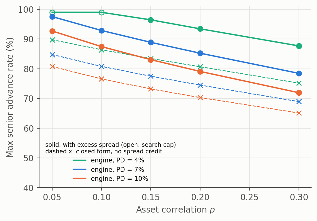
Over the grid (\(\bar p\in\{4,7,10\}\%\), \(\rho\in\{0.05,\dots,0.30\}\), 15 cells) the closed form is conservative by 6.8 to 13.0 percentage points of advance rate for the 13 cells not capped; at the base default rate of 7% the engine allows \(97.5\%\), \(92.9\%\), \(85.2\%\) and \(78.4\%\) at \(\rho=0.05\), \(0.10\), \(0.20\) and \(0.30\), against \(84.8\%\), \(80.8\%\), \(74.5\%\) and \(68.9\%\) from the closed form. The gap narrows as the default rate rises (from \(12.8\) to \(9.5\) points across the correlation range at \(\bar p=7\%\), and from \(11.9\) to \(6.8\) at \(\bar p=10\%\)), which is consistent with less excess spread being available when more of the pool defaults; we have not tested that explanation separately. Both curves fall with correlation: more correlated pools need more subordination, in the engine by roughly 3 to 5 points of advance rate per \(0.05\) of \(\rho\).
At the base parameters the pool, bought at par, has a mean unlevered IRR of \(12.3\%\) and a principal-weighted average life of \(1.29\) years. Cumulative defaults average \(8.9\%\) and net losses \(7.2\%\); across the factor distribution net losses have a 5th percentile of \(2.3\%\), a median of \(6.4\%\), a 95th percentile of \(14.6\%\) and a 99.5th percentile of \(20.7\%\). The equity cheque is \(21\%\) of the pool balance.
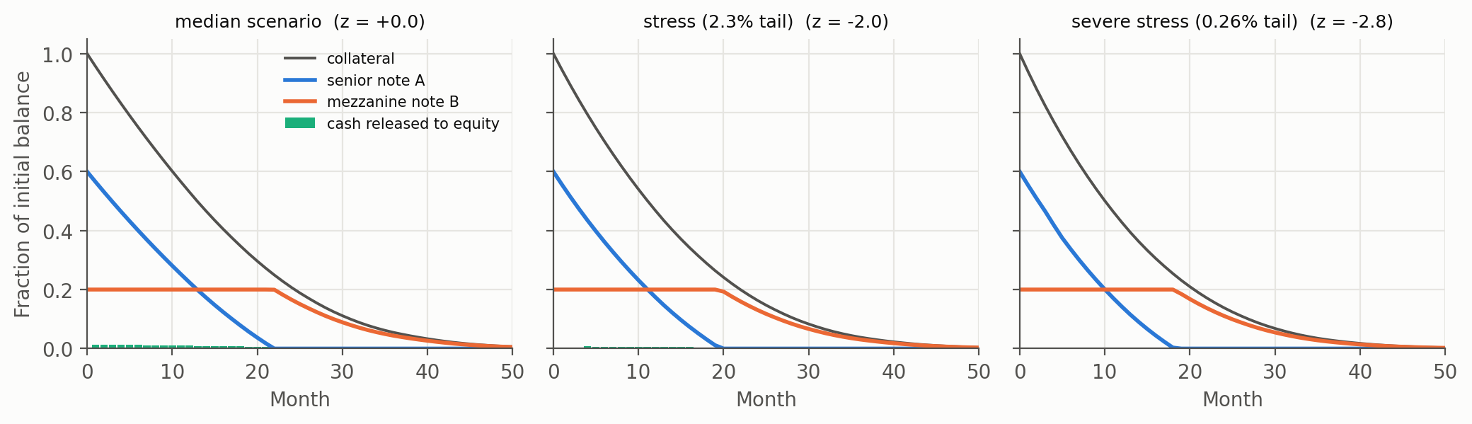
Figure 3 follows the notes and the cash released to equity through three economies. In each, the senior note amortises first; the mezzanine note stays at \(20\%\) of the original balance until the collateral has shrunk to \(B/\alpha_B\) and then amortises with it. Even in the severe scenario (0.26% tail, \(z=-2.8\)) both notes are repaid in full, because excess spread and the cash trap cover the losses.
Equity bears the risk. Its median IRR is \(26.4\%\) (5th to 95th percentile: \(-12.3\%\) to \(49.4\%\)), and it loses money in \(12.3\%\) of scenarios. Because the equity is a levered claim on the pool, its IRR is a steeper function of the economy than the pool’s: Figure 4 shows the two crossing near the 22nd percentile, below which leverage hurts. At a 20% hurdle the mean equity NPV is \(+0.44\%\) of the pool balance, about \(2.1\%\) of the cheque.
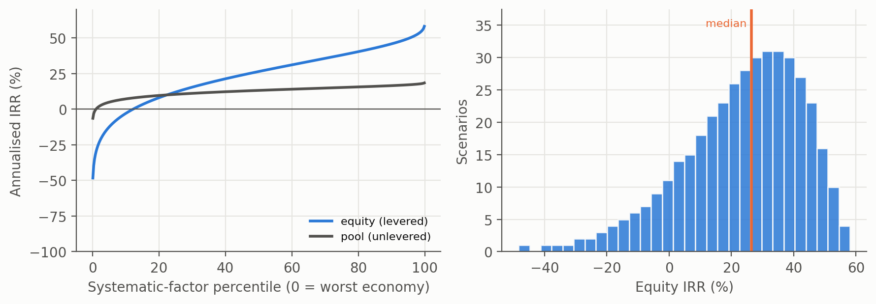
Figure 5 plots the equity NPV (left) and the probability that the equity loses money (right) over purchase price and total advance rate (\(\alpha_A=0.75\,\alpha_B\) throughout). The line where NPV is zero is the break-even price \(P^*(\alpha_B)\). It rises from \(98.3\) at a \(60\%\) advance rate to \(101.8\) at \(92\%\): each additional point of leverage lets the buyer pay about \(0.11\) points more. At the base \(80\%\) advance rate it is about \(100.4\).
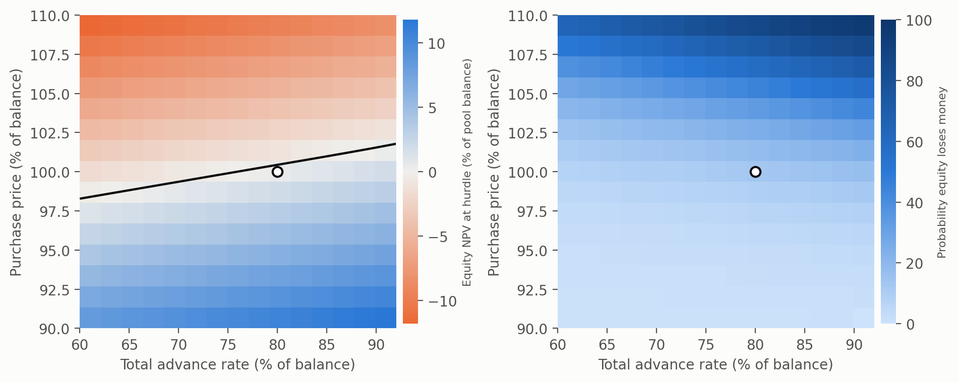
Price matters far more than leverage. Since the equity cheque is \(P+\kappa-\alpha_B\), a point of price changes the NPV by exactly one point; over the plotted range the NPV spans about \(\pm12\) points of balance, nearly all of it from price. The probability of a negative equity return, at the base advance rate, is \(3\%\) at a price of \(94\), \(12\%\) at par, \(34\%\) at \(104\) and \(72\%\) at \(109\).
We perturb each input by \(\pm10\%\) about the base case (the recovery lag by \(\pm1\) month) and report the effect of a \(+10\%\) change (a central difference, in percentage points). Because the scenario grid is deterministic there is no sampling noise. The price enters as an exact identity (\(\partial\mathrm{NPV}/\partial P=-1\)) and is omitted from the chart.
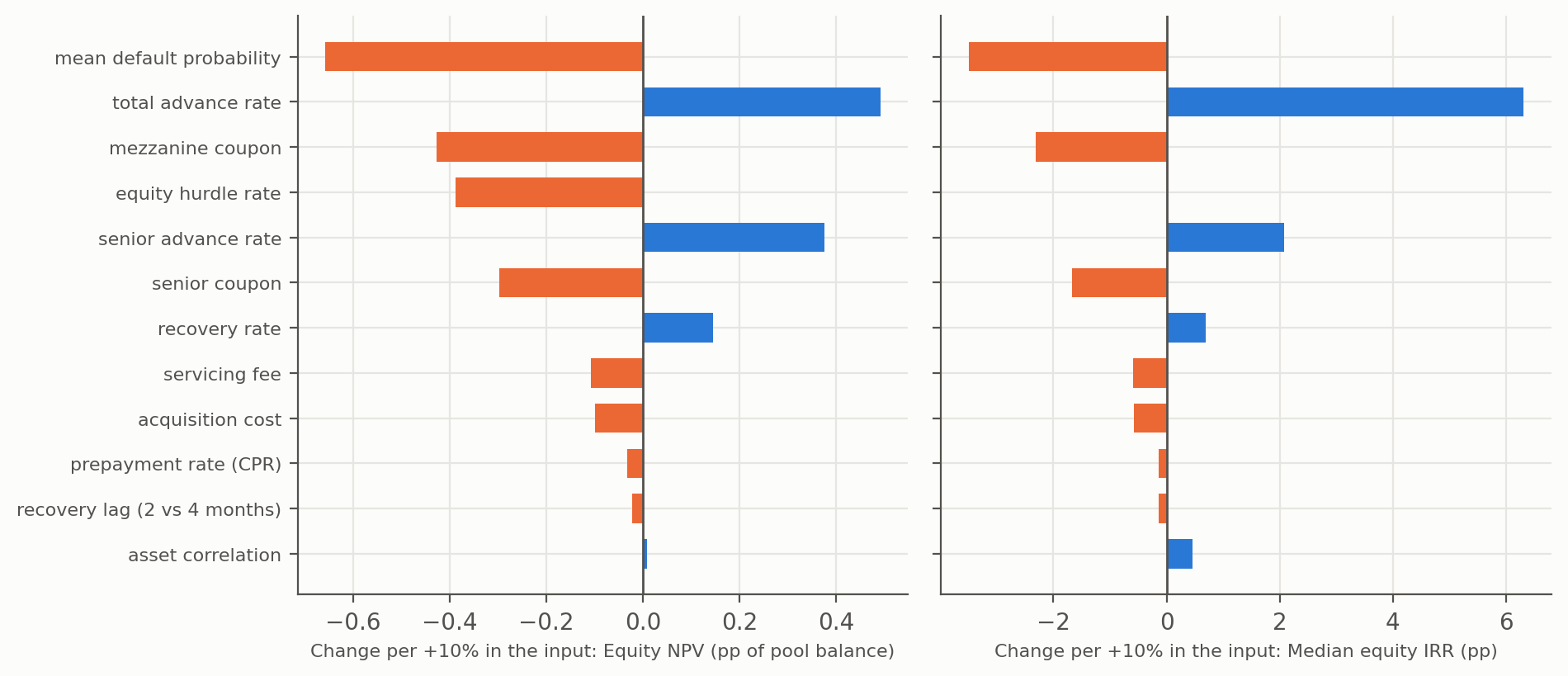
The mean default probability is the largest single driver of value: \(+10\%\) in \(\bar p\) costs \(0.66\) points of NPV and \(3.5\) points of median IRR. Leverage works the other way: \(+10\%\) in the total advance rate adds \(0.49\) points of NPV and \(6.3\) points of IRR. The mezzanine coupon (\(-0.43\)), the hurdle rate (\(-0.39\)), the senior advance rate (\(+0.38\)) and senior coupon (\(-0.30\)) follow. The recovery rate matters modestly (\(+0.14\)). Servicing and acquisition costs each cost about \(0.1\) point. The prepayment rate and the recovery lag are almost irrelevant: \(-0.03\) and \(-0.02\) points. The prepayment result is the numerical face of Corollary 1: at a price near par prepayment speed barely changes the pool’s yield, and the small residual effect on the equity NPV presumably comes from the difference between the equity’s discount rate and the pool’s yield, a point we have not isolated. The asset correlation moves the equity NPV by about \(0.01\) points but raises the probability of an equity loss by \(0.75\) points: correlation redistributes risk to the tails without changing the mean much.
A 240-point Latin-hypercube design [3] varies all 12 inputs together (each \(\pm30\%\) about the base value; advance rates \(\pm10\%\); price \(\pm8\%\)), and we summarise with partial rank correlation coefficients [4].
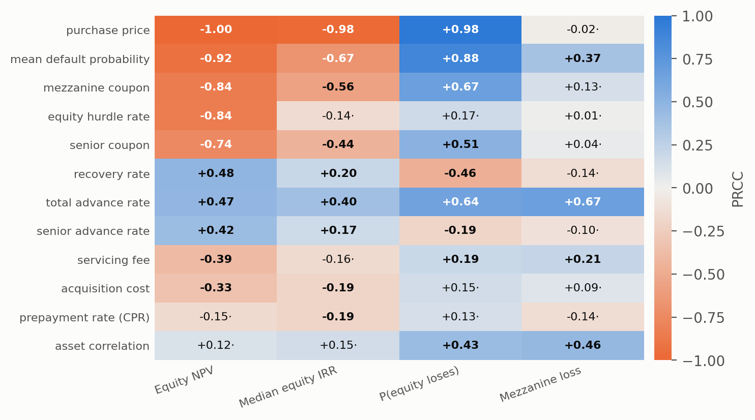
After price (\(-1.00\) for NPV), the largest effects on equity value are the mean default probability (\(-0.92\)), the mezzanine coupon (\(-0.84\)), the hurdle rate (\(-0.84\)) and the senior coupon (\(-0.74\)), then recovery (\(+0.48\)) and the two advance rates (\(+0.47\), \(+0.42\)). The ranking agrees with the one-at-a-time analysis. For the probability that equity loses money the order is price (\(+0.98\)), default probability (\(+0.88\)), mezzanine coupon (\(+0.67\)), total advance rate (\(+0.64\)) and senior coupon (\(+0.51\)); recovery lowers it (\(-0.46\)), and correlation raises it (\(+0.43\)). Mezzanine loss is driven by the total advance rate (\(+0.67\)), correlation (\(+0.46\)) and default probability (\(+0.37\)). The senior note lost no principal in any of the 240 runs (its advance rate never exceeded 66%), and the largest expected mezzanine loss was \(0.48\%\).
Propositions 1–3 are theorems about the cash-flow recursions and hold to machine precision; they apply when the notes are never short of cash. The loss law in Section 4 is an approximation, accurate to a few percent in the quantiles that matter. The sizing bound ignores excess spread by construction and is conservative by 7–13 points. Everything in Sections 5–6 is the output of the engine and inherits its assumptions.
Corollary 1 says that prepayment speed has no effect on the yield of a pool bought at par, which is set by the coupon, the default rate, the recovery and the servicing fee (prepayment still changes the timing of cash flows, and so the notes and the equity’s discounting). The price sensitivity in Corollary 3 and its leverage amplification in Corollary 4 say where a mispricing hurts: a one-point error in price is worth roughly \(5\) to \(6\) points of annualised equity IRR at an \(80\%\) advance rate (from the exact price sensitivity of Section 3), because the equity is so thin.
Synthetic data. The tape, the coupons, the hurdle and the default probabilities are illustrative; the numbers say nothing about any real pool or market.
One static factor. Systematic risk is one Gaussian factor fixed over the life. There is no time-variation, no regime change, no contagion across loans beyond the factor, and Gaussian dependence has thin joint tails.
Constant hazards. Default and prepayment rates do not depend on loan age, seasoning or the interest-rate level, and prepayment does not respond to default.
Simple structure. Two sequential-pay notes, one overcollateralisation test, no reserve account, no servicer advances, no triggers on delinquency, and fixed coupons with no interest-rate or basis risk.
The “arbitrage” is not riskless. We use the word for a positive expected equity NPV under stated assumptions and a stated hurdle. The equity loses money in \(12\%\) of scenarios at the base case.
No calibration. We did not fit any parameter to data. The closed-form loss law has one free parameter, \(\theta\), taken from the median scenario of the same engine.
Natural next steps are age-dependent default and prepayment curves, a second systematic factor for interest rates, floating-rate notes with a hedge, delinquency triggers, a closed-form for the equity NPV integrated over \(z\), and calibrating the loss law’s \(\theta\) from the pool’s amortisation schedule alone, which would make the sizing bound fully explicit.
The code is pure Python with numpy, scipy
and matplotlib. pool.py contains the synthetic
tape, the cash-flow engine and the waterfall; theory.py the
closed forms of Section 3; exp_theory.py the checks behind
Table 2; experiments.py the numerical experiments (about
four minutes on eight cores); and make_figures.py the
figures and the summary numbers quoted here. Everything is seeded and
every scenario average uses a deterministic quantile grid, so the
results reproduce exactly. The machine-readable results are in the
data/ folder of this page; the code is available from the
author on request.
[1] O. Vasicek, “Loan portfolio value,” Risk, December 2002, pp. 160–162.
M. B. Gordy, “A risk-factor model foundation for ratings-based bank capital rules,” Journal of Financial Intermediation, vol. 12, no. 3, pp. 199–232, 2003.
M. D. McKay, R. J. Beckman and W. J. Conover, “A comparison of three methods for selecting values of input variables in the analysis of output from a computer code,” Technometrics, vol. 21, pp. 239–245, 1979.
S. Marino, I. B. Hogue, C. J. Ray and D. E. Kirschner, “A methodology for performing global uncertainty and sensitivity analysis in systems biology,” Journal of Theoretical Biology, vol. 254, pp. 178–196, 2008.