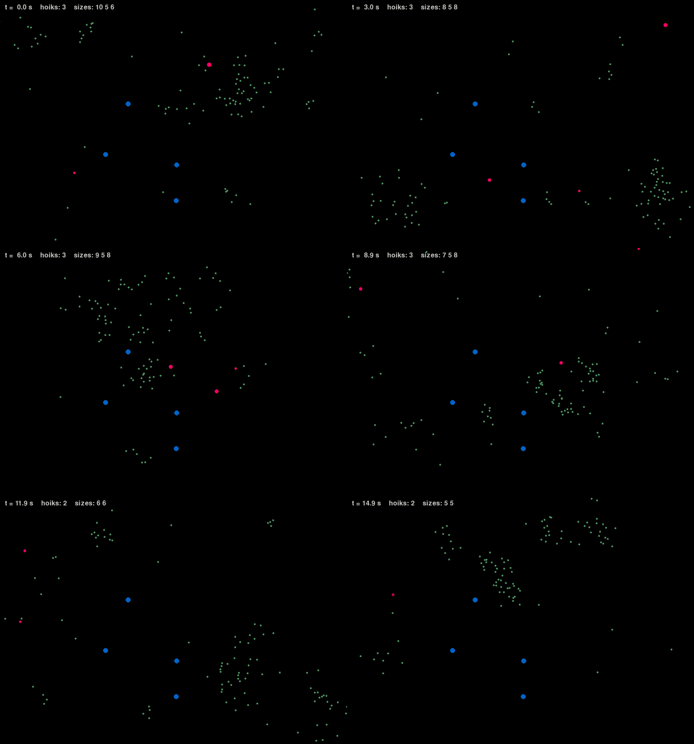
15 October 2026
We describe a small agent-based simulation in which a flock of prey (boids) is hunted by a population of predators (hoiks) in a two-dimensional arena containing static obstacles. The prey follow Reynolds’ three-rule flocking model, extended with avoidance of predators and obstacles. The predators chase the nearest prey, repel one another, and carry a simple life cycle: they grow when they feed, shrink when they starve, reproduce when large, and die when small or by chance. Growth feeds back into behaviour, because a large hoik moves much more slowly than a small one. We give the complete update rules and then analyse the model quantitatively. Instrumented headless runs show that a hoik’s size above its floor behaves like the workload of a queue: feeding contacts are the arrivals, starvation is the drain, and the speed threshold at size 10 switches the arrival rate. A two-regime diffusion approximation, whose single free quantity is the index of dispersion of the feeding process measured from the feeding log, predicts the fraction of time hoiks spend above the threshold to within sampling error at baseline (\(0.157\) predicted, \(0.146\pm0.008\) observed, though the prediction varies by a factor of two over reasonable choices of the estimation window) and predicts the decay rate of the tail above the threshold to within 5%. Coupled to a birth–death chain it predicts the hoik population less well (mean \(2.9\) against \(2.6\) observed), because the diffusion approximation understates starvation. One-at-a-time elasticities and a 120-point Latin-hypercube study identify the prey’s avoidance weight and the predators’ speed as the dominant controls of feeding, and the prey’s speed, alignment and vision radius as the controls of flock spacing and polarization. The model ranks the effect of parameter changes almost perfectly (Spearman \(\rho=0.97\)) but overstates their size by roughly a factor of three. We report these failures as results in their own right.
Flocking is one of the cleanest examples of emergence in artificial life. In 1987 Craig Reynolds showed that realistic-looking flocks, herds and schools need no leader and no global plan: each agent, which he called a boid, only reacts to its nearby neighbours using three simple rules [1]. This project asks what happens when something hunts the flock. We add a second species, the hoik, which chases boids, and give it a body size that responds to feeding. The interesting part is the feedback: hunting success makes a hoik big, and bigness makes it slow.
The simulation is written in Python with pygame and is
about 350 lines long. Sections 2–6 describe the code exactly as it runs,
including simplifications that a reader might otherwise mistake for
oversights. Section 7 then asks quantitative questions of it: how does
the predators’ size behave over time, can its statistics be predicted
from a few measured rates, and which parameters matter most?
The world is a rectangle of width \(W=1400\) and height \(H=1000\) pixels, simulated in discrete time with one step per rendered frame (60 frames per second). Time is therefore measured in frames, and “speed” means pixels per frame. There are three kinds of object.
(\(N=100\) prey). Each has a position \(\mathbf{p}_i\in\mathbb{R}^2\) and velocity \(\mathbf{v}_i\in\mathbb{R}^2\). Positions are initialised uniformly at random over the arena and velocity components uniformly in \([-1,1]\).
(predators, initially \(2\)). Each has a position, a velocity and a scalar size \(s\in[5,20]\), initially \(5\).
(\(4\) fixed discs of radius \(10\)). They are placed uniformly at random at least \(100\) pixels from every edge and never move.
Boids and hoiks share a common set of steering behaviours (Section 3); each species weights them differently.
Throughout, agent \(i\) has a vision radius \(R=100\). The neighbourhood of \(i\) is the set of other boids within vision, \[\mathcal{N}_i=\{\,j\neq i : \lVert \mathbf{p}_j-\mathbf{p}_i \rVert<R\,\}, \qquad n_i=\lvert\mathcal{N}_i\rvert .\] Each rule returns a vector; the species-specific update (below) multiplies each by a weight and sums them.
Steer toward the centre of mass of the neighbours, \[\mathbf{C}_i=\frac{1}{100}\left(\frac{1}{n_i}\sum_{j\in\mathcal{N}_i}\mathbf{p}_j-\mathbf{p}_i\right),\] and \(\mathbf{C}_i=\mathbf{0}\) if there are no neighbours. The constant \(1/100\) makes the pull proportional to distance, reaching magnitude \(1\) at the edge of vision.
Push away from anything closer than a range \(r\), \[\mathbf{S}_i(r)=-\sum_{\substack{j\ne i\\ \lVert \mathbf{p}_j-\mathbf{p}_i \rVert<r}}(\mathbf{p}_j-\mathbf{p}_i).\] The push grows linearly the closer the offender is. Boids use \(r=9\) (roughly a body length, since boids are drawn with radius \(4\)), hoiks use \(r=50\).
Match the average heading of the neighbours, \[\mathbf{A}_i=\frac{1}{8}\left(\frac{1}{n_i-1}\sum_{j\in\mathcal{N}_i}\mathbf{v}_j-\mathbf{v}_i\right),\qquad n_i>1,\] and \(\mathbf{A}_i=\mathbf{0}\) otherwise. The divisor \(n_i-1\) rather than \(n_i\) is inherited from Reynolds-style pseudocode, where it averages over the rest of the flock excluding oneself; here the neighbour set already excludes \(i\), so the average is inflated by a factor \(n_i/(n_i-1)\). The effect is small for large neighbourhoods and we have left it in place.
For a set \(\mathcal{T}\) of threats (hoiks or obstacles), flee from every one within vision, \[\mathbf{E}_i(\mathcal{T})=-\sum_{\substack{k\in\mathcal{T}\\ 0<\lVert \mathbf{p}_k-\mathbf{p}_i \rVert<R}}\hat{\mathbf{u}}_{ik}, \qquad \hat{\mathbf{u}}_{ik}=\frac{\mathbf{p}_k-\mathbf{p}_i}{\lVert \mathbf{p}_k-\mathbf{p}_i \rVert} .\] Each threat contributes a unit vector regardless of its distance, so avoidance is all-or-nothing within the vision radius. This rule also carries the model’s collision mechanic: if agent \(i\) comes within the size of a threat, \(\lVert \mathbf{p}_k-\mathbf{p}_i \rVert<\sigma_k\), then \(i\) is teleported to a uniformly random point in the arena. For an obstacle \(\sigma=10\); for a hoik, \(\sigma=s\).
Move straight toward the closest boid within vision, \[\mathbf{P}_h=\hat{\mathbf{u}}_{h,j^\star},\qquad j^\star=\arg\min_{j:\ \lVert \mathbf{p}_j-\mathbf{p}_h \rVert<R}\lVert \mathbf{p}_j-\mathbf{p}_h \rVert,\] and \(\mathbf{P}_h=\mathbf{0}\) if no boid is in sight.
After moving, any agent within \(m=100\) pixels of an edge has its velocity nudged by \(0.7\) back toward the interior along that axis. For example, if \(x>W-m\) then \(v_x\leftarrow v_x-0.7\); there are four such cases. This is a steering force, not a wall, so a fast agent can overshoot the margin, and the nudge takes effect at the next step. (A wrap-around alternative exists in the source but is not used.)
Each frame, boid \(i\) computes its neighbourhood and then updates its velocity as \[\begin{equation} \label{eq:boid} \mathbf{v}_i\leftarrow \mathbf{v}_i + 0.2\,\mathbf{C}_i + 0.4\,\mathbf{S}_i(9) + 0.3\,\mathbf{A}_i + 0.6\,\bigl[\mathbf{E}_i(\mathcal{H})+\mathbf{E}_i(\mathcal{O})\bigr], \end{equation}\] where \(\mathcal{H}\) is the set of hoiks and \(\mathcal{O}\) the set of obstacles. The velocity is then renormalised to a fixed speed and applied, \[\begin{equation} \label{eq:speed} \mathbf{v}_i\leftarrow 5\,\frac{\mathbf{v}_i}{\lVert \mathbf{v}_i \rVert},\qquad \mathbf{p}_i\leftarrow\mathbf{p}_i+\mathbf{v}_i, \end{equation}\] followed by the soft boundary rule.
Two consequences of the speed normalisation are worth stating. First, the model has no inertia in the physical sense: the steering terms change a boid’s direction but never its speed, which is always \(5\). To first order, a steering vector of magnitude \(F\) perpendicular to the heading rotates it by roughly \(\arctan(F/5)\) per frame; one full-strength avoidance term (\(0.6\)) turns a boid by about \(7^\circ\) per frame. Second, the weights in the velocity update are best read as gains relative to a speed of \(5\), not as probabilities or fractions.
Updates are applied sequentially within a frame. When boid \(i\) is updated it sees the already-moved positions of boids \(1,\dots,i-1\) and the old positions of the rest. This asynchronous scheme is common in hobbyist simulations and removes the need to double-buffer state, at the price of a very slight order dependence.
A hoik’s life has two parts: a size-changing life cycle and a movement rule that depends on size.
Hoiks follow \[\begin{equation} \label{eq:hoik} \mathbf{v}_h\leftarrow \mathbf{v}_h + 0.7\,\mathbf{P}_h + 0.5\,\mathbf{S}_h(50) + 0.4\,\mathbf{A}^{\text{all}}_h + 1.0\,\mathbf{E}_h(\mathcal{O}), \end{equation}\] where \(\mathbf{S}_h(50)\) is separation among hoiks (to stop predators piling onto one prey) and \(\mathbf{A}^{\text{all}}_h\) is the alignment rule applied to all boids rather than only those in vision, so hoiks are gently biased toward the flock’s mean velocity. The velocity is then renormalised as for boids, but with a size-dependent speed \[\begin{equation} \label{eq:hoikspeed} \lVert\mathbf{v}_h\rVert= \begin{cases} 7, & s\le 10,\\ 2, & s>10, \end{cases} \end{equation}\] so that small hoiks are faster than boids (\(7>5\)) and large ones are much slower (\(2<5\)). This is the central trade-off of the model.
Capture is implemented as two separate events that happen to be triggered by proximity:
Hoik growth. For each boid \(j\) with \(\lVert \mathbf{p}_j-\mathbf{p}_h \rVert<s+2\), the hoik gains \(1\) unit of size, capped at \(20\). The check is made boid by boid, so the reach \(s+2\) grows during the loop.
Boid respawn. A boid with \(\lVert \mathbf{p}_h-\mathbf{p}_j \rVert<s\) is teleported to a random location by the avoidance rule above.
Because the reach for feeding (\(s+2\)) is larger than the kill radius (\(s\)), the two events are not perfectly synchronised: a boid hovering just outside the kill radius can feed a hoik repeatedly without being removed, and a boid can occasionally be teleported without feeding the hoik. The boid population is therefore constant at \(N=100\); predation never depletes the prey, and the model deliberately has no prey birth–death dynamics.
Every frame the hoik also loses a little size, \[s\leftarrow\max(5,\,s-0.01),\] so a hoik that stops feeding shrinks from \(20\) to \(10\) in \(1000\) frames (about \(17\) seconds) and recovers its speed advantage. To merely hold its size, a hoik needs to feed on average once every \(100\) frames.
Population control follows simple stochastic rules evaluated every frame for every hoik. Let \(\lvert\mathcal{H}\rvert\) be the current number of hoiks.
Reproduction. If \(\lvert\mathcal{H}\rvert<10\) and \(s>10\), with probability \(10^{-3}\) the hoik spawns a new hoik (of size \(5\)) within one pixel of itself. Parents lose nothing. The expected wait is \(1000\) frames.
Starvation death. If \(\lvert\mathcal{H}\rvert>2\) and \(s<6\), with probability \(5\times10^{-4}\) the hoik dies.
Background death. If \(\lvert\mathcal{H}\rvert>2\), with probability \(10^{-4}\) any hoik dies regardless of size (the source comments call this a “heart attack”).
The condition \(\lvert\mathcal{H}\rvert>2\) means the population never falls below two, which keeps the simulation from ending in extinction.
Note the interplay of the size-dependent speed and the reproduction threshold. To breed, a hoik must exceed size \(10\), which needs a good run of kills; but once above \(10\) it becomes slow (\(2<5\)) and can no longer outrun a boid in open water. It can still catch prey that drift toward it, that are cornered by obstacles or the arena margin, or that are pushed past it by the flock. This negative feedback tends to keep the predators from simply growing without bound.
| Quantity | Symbol / location | Value |
|---|---|---|
| Arena | \(W\times H\) | \(1400\times1000\) |
| Frame rate | 60 | |
| Boids / initial hoiks / obstacles | 100 / 2 / 4 | |
| Vision radius (all agents) | \(R\) | 100 |
| Boid speed | 5 | |
| Hoik speed (\(s\le10\) / \(s>10\)) | 7 / 2 | |
| Boid weights: cohesion, separation, alignment, avoidance | 0.2, 0.4, 0.3, 0.6 | |
| Boid separation range | \(r\) | 9 |
| Hoik weights: pursuit, separation, alignment, obstacles | 0.7, 0.5, 0.4, 1.0 | |
| Hoik separation range | \(r\) | 50 |
| Hoik size range, feeding reach | \([5,20]\), \(s+2\) | |
| Shrink rate | 0.01 / frame | |
| Reproduction (size \(>10\), \(\lvert\mathcal{H}\rvert<10\)) | \(10^{-3}\) / frame | |
| Death (size \(<6\), \(\lvert\mathcal{H}\rvert>2\)) | \(5\times10^{-4}\) / frame | |
| Death (any size, \(\lvert\mathcal{H}\rvert>2\)) | \(10^{-4}\) / frame | |
| Boundary margin / nudge | \(m\) | 100 / 0.7 |
Every boid scans all other boids to find its neighbours, so a frame costs \(O(N^2)\) distance evaluations (about \(10^4\) for \(N=100\)) plus \(O(N\lvert\mathcal{H}\rvert)\) for the predators. This is entirely adequate at this scale; scaling to thousands of agents would call for a spatial hash or grid.
All experiments run the repository’s own Boid,
Hoik and Obstacle classes headlessly, without
drawing. The only additions are passive observers: a thin subclass of
Hoik that logs each \(+1\)
jump in size (a feeding contact, tagged by the speed regime it
occurred in), and per-frame bookkeeping of births, deaths and teleports.
The parameters in Table 1 that we vary were turned into class
attributes; with default values the instrumented code reproduces an
unmodified seeded run exactly. We measure:
Flock structure: polarization \(\Phi=\lVert N^{-1}\sum_i \mathbf{v}_i/\lVert\mathbf{v}_i\rVert\rVert\in[0,1]\) and the mean nearest-neighbour distance.
Feeding: the contact rates \(\lambda_f\) (while \(s\le10\)) and \(\lambda_s\) (while \(s>10\)), in contacts per hoik per frame, and the capture rate (boids teleported by a hoik, per hoik per frame).
Hoik state: the fraction of hoik-time spent with \(s>10\), the distribution of sizes, and the number of hoiks.
Every run discards an initial transient before accumulating statistics, because hoiks start at the minimum size and boids start scattered. An early version of this study omitted that step, and it biased the sensitivity runs: the fraction of time above size 10 comes out systematically high in short runs. The three experiments are:
24 seeds \(\times\) 14 000 frames (about 233 s), first 2 500 frames discarded.
Each of the 11 parameters shown in Figure 5 set to \(0.75\times\) and \(1.25\times\) its default, 6 seeds each, plus 6 baseline seeds, 10 000 frames, first 3 000 discarded.
A 120-point Latin hypercube over all 11 parameters simultaneously, each scaled uniformly in \([0.6,1.4]\) times its default, one run per point, 8 000 frames, first 2 500 discarded.
Uncertainties are 95% bootstrap intervals over seeds unless stated otherwise.
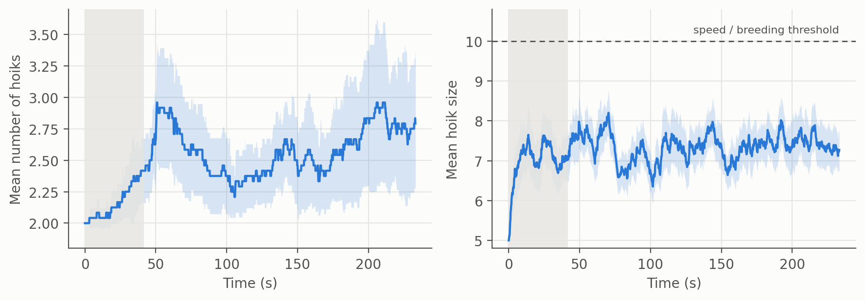
At default parameters the flock is moderately aligned (polarization \(0.341\pm0.006\)) and loosely packed (mean nearest-neighbour distance \(30.7\pm0.1\) px, against a vision radius of \(100\) px). The hoiks usually number two, occasionally three or four (time-average \(2.58\pm0.12\)), and spend most of their time small and fast. Figure 2 shows the time course: the mean hoik size rises from the floor of \(5\) in the first seconds and then settles at about \(7.4\) and does not approach the threshold at \(10\) on average.
Hoiks are not well fed on average. A small hoik makes \(\lambda_f=0.00773\) feeding contacts per frame (95% interval \(0.00745\) to \(0.00802\)), which is below its shrink rate \(\delta=0.01\) per frame. Define the load \[\rho=\lambda_f/\delta=0.773\;(0.745\text{ to }0.802),\] the ratio of how fast a small hoik feeds to how fast it starves. Because \(\rho<1\) a small hoik does not grow without bound; it is held near the floor and only occasionally rises. Large hoiks feed more slowly, \(\lambda_s=0.00612\) (\(0.00572\) to \(0.00647\)), because their speed drops from \(7\) to \(2\) and boids easily outrun them. The next section shows that these two rates and one measure of burstiness are enough to predict how the size is distributed.
Let \(x=s-5\ge0\) be a hoik’s size above the floor. Feeding contacts add \(1\) to \(x\); starvation removes \(\delta\) per frame; the floor makes \(x\) reflect at zero. If contacts arrived as a Poisson process with rate \(\lambda\) this is exactly the workload of an M/D/1 queue with load \(\rho=\lambda/\delta\), and its stationary law is Erlang’s: \[P(x\le y)=(1-\rho)\sum_{k=0}^{\lfloor y\rfloor}\frac{\bigl(-\rho(y-k)\bigr)^k}{k!}e^{\rho(y-k)} .\] This predicts that a hoik spends \(P(s>10)=P(x>5)=7.2\%\) of its time above the threshold at \(\rho=0.773\). The simulation gives \(14.6\pm0.8\%\). The prediction is a factor of two too low, and the reason is visible in the feeding log.
A boid that lingers inside a hoik’s reach feeds it on consecutive frames. Of all gaps between successive contacts of the same hoik, \(39\%\) are one frame or less, and a maximal run of consecutive-frame contacts (a burst) contains on average \(1.60\) contacts. If bursts arrived independently, the size process would be an M/G/1 workload and the Pollaczek–Khinchine formula would apply exactly, \[P(x\le y)=(1-\rho)\sum_{n\ge0}\rho^n H^{*n}(y),\] where \(H\) is the equilibrium law of the burst size. With the measured burst distribution this predicts \(31.1\%\), now a factor of two too high. Neither exact formula is right, so the arrivals must be neither Poisson nor independent bursts.
The discrepancy is explained by the index of dispersion \(F(W)=\mathrm{Var}\,N_W/\mathrm{E}\,N_W\) of the contact count \(N_W\) in windows of \(W\) frames, measured from every window that lies inside one hoik’s lifetime (Table 2). Independent bursts would give \(F=\mathrm{E}[K^2]/\mathrm{E}[K]=2.49\) at every window length. Instead \(F\) starts there and falls steadily as the window grows. At long windows feeding is more regular than independent bursts, which is what one expects if a hoik that has just fed has depleted the prey around it: a refractory effect. Because the size process integrates feeding over times of order \(\sigma^2/\mu^2\sim\) one to two thousand frames, it is the long-window value that matters.
| Window \(W\) (frames) | Windows | \(F(W)\) | Predicted \(P(s>10)\) |
|---|---|---|---|
| 50 | 14 113 | 2.60 | 0.219 |
| 100 | 7 019 | 2.59 | 0.218 |
| 200 | 3 460 | 2.49 | 0.207 |
| 400 | 1 684 | 2.30 | 0.185 |
| 800 | 804 | 2.06 | 0.157 |
| 1600 | 371 | 1.72 | 0.115 |
We therefore replace the jump process by the diffusion with the same drift and variance rate. In regime \(r\in\{f,s\}\) (below and above the threshold) the drift of \(x\) is \(\mu_r=\lambda_r-\delta\) and the variance rate is \(\sigma_r^2=\lambda_r F\). The stationary density of a reflected diffusion is \(\pi(x)\propto\sigma^{-2}(x)\exp\!\int_0^x 2\mu/\sigma^2\), which here is piecewise exponential, \[\pi(x)\propto \begin{cases} \dfrac{e^{-\theta_f x}}{\lambda_f F}, & 0\le x<5,\\[2ex] \dfrac{e^{-5\theta_f}e^{-\theta_s(x-5)}}{\lambda_s F}, & x\ge5, \end{cases} \qquad \theta_r=\frac{2(\delta-\lambda_r)}{\lambda_r F},\] with \(\theta_f\) allowed to be negative. Integrating gives closed forms for every quantity of interest, for example \[P(s>10)=\frac{e^{-5\theta_f}/(\theta_s\lambda_s)}{(1-e^{-5\theta_f})/(\theta_f\lambda_f)+e^{-5\theta_f}/(\theta_s\lambda_s)},\] and the size tail above \(10\) decays as \(e^{-\theta_s(s-10)}\). The model has no fitted parameters: \(\lambda_f\), \(\lambda_s\) and \(F\) are all measured from the feeding log, and none is tuned to the size distribution.
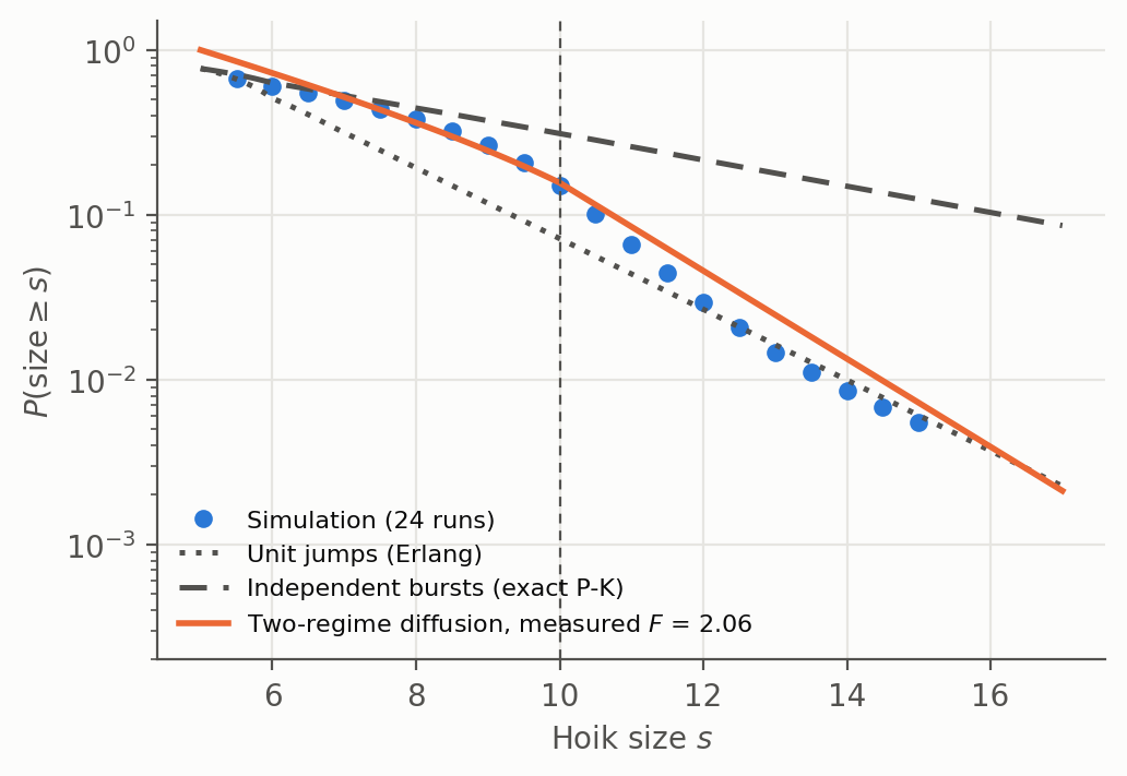
Figure 3 and Table 3 compare the models with the simulation. At the baseline the two-regime model predicts \(P(s>10)=0.157\) (interval \(0.116\) to \(0.200\), from sampling error in \(\lambda_f\) and \(F\)), against \(0.146\pm0.008\) observed. It also predicts the decay rate of the tail above the threshold: \(\theta_s=0.615\) predicted against \(0.650\) measured by regression over sizes \(10.5\) to \(15\) (5% low), a check that uses the slow-regime feeding rate and not the quantity the model was calibrated on. The weak points are in the lower tail: it predicts \(P(s<6)=0.275\) where \(0.396\) is observed, because a diffusion has no probability atom at the floor, whereas simulated hoiks do pile up at the minimum size.
Table 2 shows the weakest link. The prediction depends on the window used to estimate \(F\), and over the range of windows we could estimate it, it moves between \(0.115\) and \(0.219\). We used \(W=800\), the longest window that was well sampled in our first analysis. With the larger re-run data \(W=1600\) is also reasonably well sampled and would give a prediction below the observed value, so the agreement at baseline should be read as “within the plausible range” and not as a precise confirmation.
| Model | \(P(s>10)\) | Comment |
|---|---|---|
| Simulation (observed) | \(0.146\pm0.008\) | |
| M/D/1 (Poisson unit jumps) | 0.072 | ignores bursts |
| M/G/1 (independent bursts) | 0.311 | ignores regularity |
| Single-regime heavy traffic | 0.186 | ignores the slow regime |
| Two-regime diffusion, \(F(800)\) | 0.157 | no fitted parameters |
The size distribution determines the demographic rates. A hoik is eligible to breed while \(s>10\) and is exposed to starvation death while \(s<6\). Per hoik per frame the birth rate is \(\beta\,P(s>10)\) with \(\beta=10^{-3}\), and the death rate is \(\mu_0+\mu_s\,P(s<6)\) with \(\mu_0=10^{-4}\), \(\mu_s=5\times10^{-4}\), the latter only when more than two hoiks exist. With the count \(H\) confined to \(\{2,\dots,10\}\), this is a birth–death chain with \[\frac{\pi(H+1)}{\pi(H)}=\frac{H\,b(H)}{(H+1)\,d(H+1)},\] where the load \(\rho\) is taken from the measured feeding rate at each \(H\).
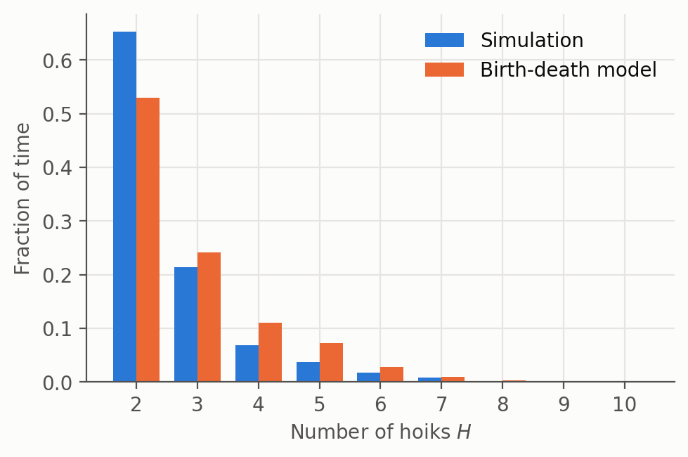
The chain gets the demographic rates about right and the population only approximately. The measured birth rate is \(1.63\times10^{-4}\) per hoik-frame against \(1.57\times10^{-4}\) predicted. The measured death rate is \(1.52\times10^{-4}\) against \(1.17\times10^{-4}\), an underestimate of about 23%, inherited from the understated starvation probability. The model therefore keeps too many hoiks (Figure 4): mean \(2.89\) against \(2.58\pm0.12\) observed, and time at the minimum of two hoiks \(0.53\) against \(0.65\). The two exact queue formulas bracket the answer wildly (means of \(2.18\) and \(4.54\)), so the diffusion model is a real improvement, but it is not accurate to better than about \(12\%\) here.
For each parameter \(\vartheta\) and output \(y\) we compute the elasticity \(\varepsilon=\partial\ln y/\partial\ln\vartheta\) from the \(\pm25\%\) runs (a central difference in the logarithm), with bootstrap intervals over seeds. Table 4 gives the six parameters with the largest effects, and Figure 5 shows all 11 parameters on 5 outputs.
| Parameter | Feeding rate \(\lambda_f\) | Time with \(s>10\) | Predicted, time \(s>10\) | |
|---|---|---|---|---|
| boid avoidance weight | \(-1.83^{*}\) | \(-3.22^{*}\) | \(-9.5\) | |
| hoik speed (small) | \(+1.32^{*}\) | \(+2.18^{*}\) | \(+8.3\) | |
| boid speed | \(+0.51^{*}\) | \(+2.78^{*}\) | \(+6.4\) | |
| hoik pursuit weight | \(+1.07^{*}\) | \(+1.08^{*}\) | \(+4.2\) | |
| boid alignment weight | \(+0.31^{*}\) | \(+0.68^{*}\) | \(+2.2\) | |
| hoik shrink rate | \(-0.20\) | \(-3.07^{*}\) | \(-6.3\) |
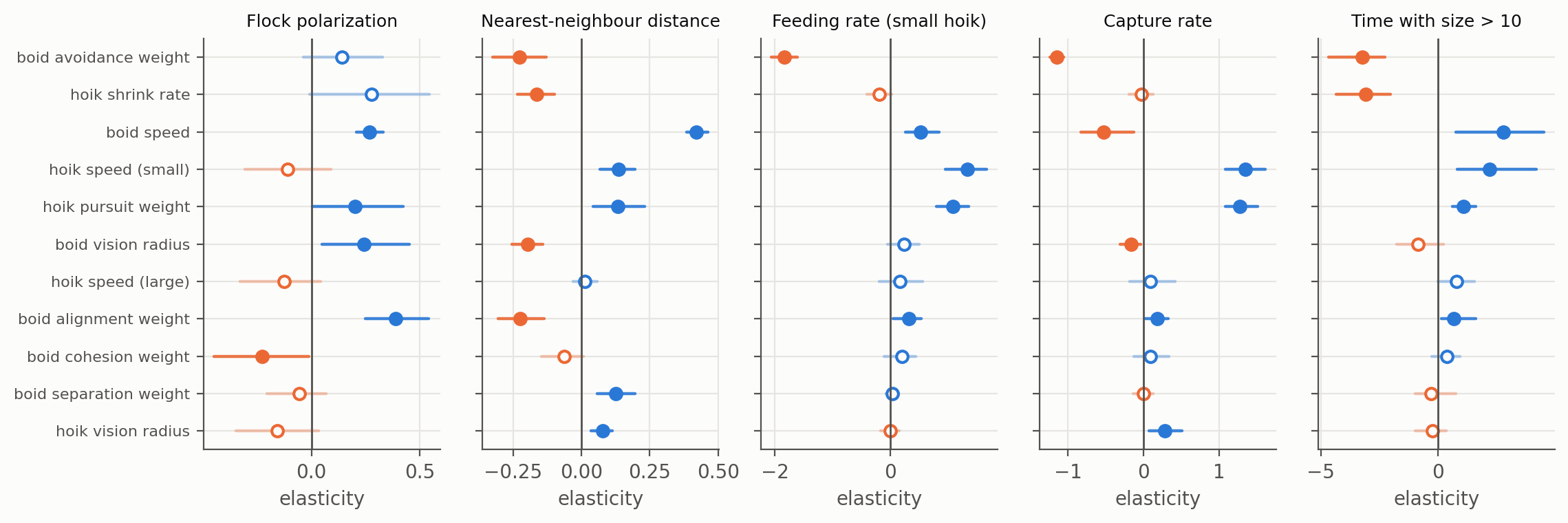
The elasticities show how steeply the outcome responds to hunting efficiency. A 1% change in the boids’ avoidance weight changes the feeding rate by \(-1.8\%\) and the time hoiks spend above size \(10\) by \(-3.2\%\): effects on the hoiks’ fate are amplified about 1.8-fold over the effect on the feeding rate that causes them, because the tail of the size distribution is exponentially sensitive to the load.
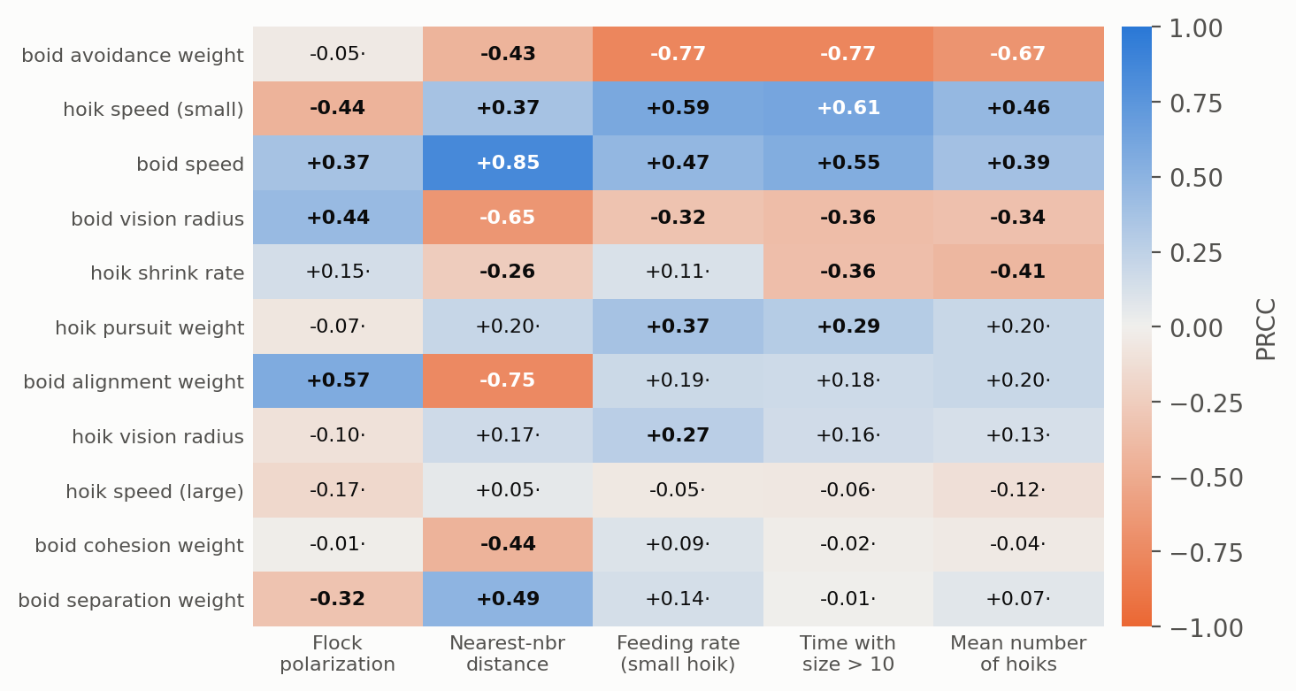
The Latin-hypercube study varies all parameters together. Figure 6 shows partial rank correlation coefficients (PRCC), which measure the monotone effect of each parameter after removing the linear effect of the others. Bold entries have \(p<0.01\).
Two groups of parameters control two separate things.
Predation success is set by the prey’s avoidance weight (\(\mathrm{PRCC}=-0.77\) for both feeding rate and time above size \(10\)), the hoiks’ small-size speed (\(+0.59\), \(+0.61\)), the prey’s speed (\(+0.47\), \(+0.55\)) and the pursuit weight (\(+0.37\) for feeding). These same parameters, together with the shrink rate (\(-0.41\)), control the number of hoiks.
Flock geometry is set by the prey’s own rules. The nearest-neighbour distance is dominated by prey speed (\(+0.85\)), alignment weight (\(-0.75\)) and vision radius (\(-0.65\)); polarization by alignment weight (\(+0.57\)) and vision (\(+0.44\)). Predator parameters have little effect on spacing, with one exception: a faster, more aggressive predator raises polarization (elasticities \(+1.3\) for small-hoik speed and pursuit).
The large-hoik speed has no significant effect on any output (presumably because large hoiks are rare); the cohesion weight affects only the nearest-neighbour distance (\(-0.44\)); the hoiks’ vision radius only slightly affects feeding (\(+0.27\)).
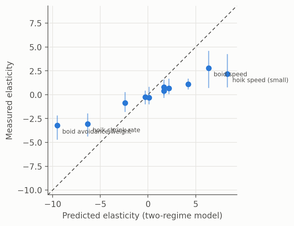
The two-regime model turns a measured change in the feeding rates into a predicted change in the time above the threshold. Across the 11 parameters the predicted and measured elasticities agree very well in ordering (Spearman \(\rho=0.97\), Pearson \(0.98\)) but not in size: the measured elasticities are on average \(35\%\) of predicted (slope of measured on predicted), and only 2 of the 11 predictions fall within the measured 95% interval (Figure 7).
Across all \(23\) one-at-a-time configurations the predicted time above the threshold again correlates strongly with the observed (Pearson \(0.93\), Spearman \(0.94\)) but is biased high at the top of the range (mean absolute error \(0.070\); the fitted slope of observed on predicted is \(0.43\)). For the \(120\) single runs of the global study the Spearman correlation is \(0.94\) and the mean absolute error is \(0.150\) (Figure 8).
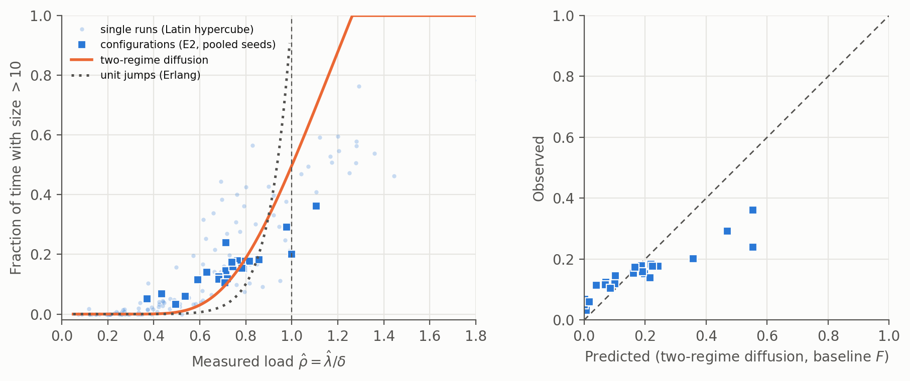
Four limitations stand out. First, the dispersion \(F\) is not a universal constant: it is a property of how the hoiks’ hunting interacts with flock geometry, and we measured it only at the baseline. When a parameter change alters it, the model predicts the right direction and ranking but the wrong magnitude, which is the pattern in Figures 7 and 8. In an exploratory first-pass batch on a pursuit-by-avoidance grid (short runs made before the burn-in fix, which we stopped before it could be re-run and so do not report in detail) \(F\) varied between \(1.2\) and \(3.4\) across settings, which supports this explanation but does not prove it. Second, the diffusion approximation ignores the probability atom at the minimum size, so it understates starvation and, through the birth–death chain, the death rate. Third, the supercritical regime, where \(\rho>1\) and a small hoik grows until it slows down at the threshold and then hovers there, is a theoretical consequence of the model (for \(F\to0\) the fraction of time above the threshold tends to \((\lambda_f-\delta)/(\lambda_f-\lambda_s)\)), but only one of our 23 configurations had \(\hat\rho\) above \(1.05\), so it is essentially untested here. Fourth, six seeds per setting give wide intervals: the one-at-a-time elasticities of the time above size \(10\) have intervals of order \(\pm2\) for several parameters, so only the strongest effects are individually established.
The simulation is deliberately simple, and several of its design choices matter for what follows from it.
Prey are never depleted. Boids hit by a hoik reappear at random, so there is no Lotka–Volterra-style oscillation. The only population that varies is that of the predators, regulated by feeding rate and the random birth–death rules rather than by prey scarcity. This is why a queue model with an infinite prey supply works at all.
Decoupled capture. Feeding and removal are independent proximity tests with different radii (\(s+2\) and \(s\)). This is what creates bursts of contacts, and the bursts are what break the simplest queueing model.
Pursuit is purely greedy. Hoiks target the nearest visible boid and have no prediction or memory.
Threat response is unweighted by distance. A hoik at the edge of vision repels as strongly as one at close range.
Global hoik alignment. Hoiks align with the whole flock, not just with prey in sight, a modelling convenience rather than a biological claim.
Parameters were chosen by eye. The weights were not calibrated against data; the sensitivity analysis is intended to tell a reader which of them are worth tuning.
The quantitative picture is that the hoik’s life is governed by a single dimensionless ratio, the load \(\rho=\lambda_f/\delta\) of feeding rate to starvation rate, and by one measure of how bursty and regular the feeding is. The baseline sits at \(\rho\approx0.77\), comfortably below the critical value of one, and the system is highly sensitive to it: the model gives an elasticity of the time above the threshold with respect to the feeding rate of about \(4.4\) at the one-at-a-time operating point, although the measured ratios in Table 4 range from about \(1\) to \(5\). This is why modest changes to the prey’s avoidance or the predators’ speed so strongly change how many hoiks the arena supports. Natural extensions include atomic predation with prey reproduction (to recover classical predator–prey cycles), a model of how the dispersion \(F\) depends on the flock’s geometry, a boundary correction to the diffusion that restores the atom at the floor, a spatial index for larger populations, and a re-run of the pursuit-by-avoidance grid with the burn-in fix, to test the supercritical regime.
The code requires Python 3 and pygame. From the
repository root, run pip3 install pygame followed by
python3 main.py. A window opens showing boids as small
green discs, hoiks as pink discs whose radius equals their size, and
obstacles as blue circles.
The experiments need numpy, scipy and
matplotlib in addition. From the experiments
folder, python run_experiments.py e1 (and e2,
e3) reproduces the three data sets, which are written to
results/; analysis_e1.py and
analysis_sens.py produce every figure and the summary
tables as JSON; mathmodels.py contains all analytic
formulas used in this paper; and render_clip.py renders the
animation. Runs are seeded, so results are reproducible bit for bit on
the same Python and pygame versions. Several of the results
above are sensitive to the choices described in Section 7.1 (burn-in
length, the window used to estimate \(F\)), and we encourage readers to vary
them.
[1] C. W. Reynolds, “Flocks, herds and schools: A distributed behavioral model,” Computer Graphics (SIGGRAPH ’87 Proceedings), vol. 21, no. 4, pp. 25–34, 1987. J. F. C. Kingman, “The single server queue in heavy traffic,” Proc. Cambridge Philos. Soc., vol. 57, pp. 902–904, 1961.
S. Asmussen, Applied Probability and Queues, 2nd ed., Springer, 2003.
S. Marino, I. B. Hogue, C. J. Ray and D. E. Kirschner, “A methodology for performing global uncertainty and sensitivity analysis in systems biology,” J. Theor. Biol., vol. 254, pp. 178–196, 2008.
M. D. McKay, R. J. Beckman and W. J. Conover, “A comparison of three methods for selecting values of input variables in the analysis of output from a computer code,” Technometrics, vol. 21, pp. 239–245, 1979.